Try it for yourself!

You can try out Flickr’s Magic View on your own photos here, and you can download a working code sample of the simplified lambda architecture here: https://github.com/yahoo/simplified-lambda

Introduction

In this post we’re going to talk about how we came up with a novel revision of the Lambda Architecture for fusing large-scale bulk compute with streaming compute to power Flickr’s Magic View. We were able to create a responsive, real time database operating at a scale of tens of billions of records, with tens to hundreds of millions of records updated per day. We turned to Yahoo’s Hadoop stack to find a way to build this at the massive scale we needed.

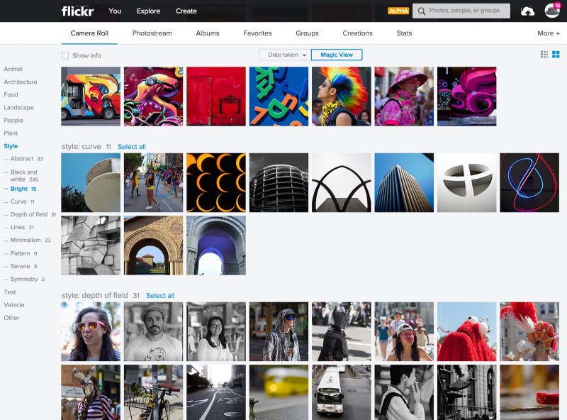
Figure 1. Magic View in action

Motivation: the Magic View

Flickr’s Magic View takes the hassle out of organizing your photos by applying our computer-vision technology to automatically recognize objects or styles in your photos and present them to you in the Camera Roll’s scrolling view. This all happens in real time — as soon as a photo is uploaded, it is categorized and placed into the Magic View.

Aggregating computer vision tags

When a photo is uploaded, it is processed by a computer vision pipeline to generate a set of computer vision tags, which are text labels of the contents of the image. We already had an existing architecture for stream computation of tags on upload, but to implement the Magic View, we needed to maintain per-user reverse indexes and some aggregations of the tags. And we needed to make sure all the data was consistent — if a photo was added, removed or updated these indexes and aggregations would have to be updated to reflect this. Finally, we needed to initialize the system with tags for 12 billion photos and videos and run periodic backfills (every time we improved our computer vision algorithms and to cover cases where the stream compute missed images).

The Problem

We initially computed a snapshot of the Magic View indexes and aggregations using map-reduce (via Apache Oozie and Apache Pig), and we were happy with the quick turnaround time (about 7 hours). We considered updating Magic View as a daily batch job, but soon realized this would not give our users the responsive, “live” experience we wanted. So, we built a streaming data layer using Apache Storm and were soon able to update the categories in Magic View in real-time.

The next time we needed to run a backfill, we explored using this streaming layer to load the data. Unfortunately, the overhead of the read-modify-write process was simply too much for a load of this size — after kicking off the process we estimated it would take 28 days this way — much longer than the seven hours we had achieved with a bulk load.

Twenty-eight days was a non-starter – we realized we needed a way to update our bulk aggregations independently of the real-time data streaming in. Solving this problem is how we arrived at our revision to Lambda Architecture. Before digging into the solution, let’s do a quick review of the Lambda Architecture.  If you’re already familiar with it, you can skip this next section.

The Lambda Architecture

We’ll start with Nathan Marz’s book ‘Big Data’, which proposes the database concept of  ‘Lambda Architecture.’ In his analysis, he states that a database query can be represented as a function – Query – which operates on all the data:

result = Query(all data)

In the Lambda architecture, a traditional database is replaced with both a real time and a bulk database. Then query function becomes a “combiner” function of independent queries to each database:

result = Combiner(Query(real time data) + Query(bulk data))

An example of a typical Lambda Architecture is shown in figure 2. It is powered by an append-only queue for its system of record, which is fed by a real time stream of events. Periodically, all the data in the queue is fed into a bulk computation which pre-processes the data to optimize it for queries, and stores these aggregations in a bulk compute database. The real time event stream drives a stream computer, which processes the incoming events into real time aggregations. A query then goes via a query combiner, which queries both the bulk and real time databases, computes the combination, and stores the result.

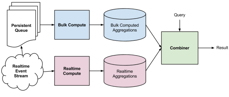
Figure 2. Typical Lambda Architecture

While relatively new, Lambda Architecture has enjoyed popularity and a number of concrete implementations have been built. Some significant examples are the distributed analytics platform druid, Twitter’s Summingbird, and FiloDB. These implementations conveniently abstract away the databases behind the query combiner.

A significant advantage with this style of architecture is robustness and fault-tolerance via eventual consistency. If a piece of data is skipped in the real time compute there is a guarantee that it will eventually appear in the bulk compute database.

Criticism of the Lambda Architecture has centred around the complicated nature of the combiner. The combiner incurs a developer and systems cost from the need to maintain two different databases. It can be challenging to make sure both systems give the same result. Merging the two queries can become complicated, and finally, more points of failure may be introduced.

The “Ah-ha” Moment

Back to the problem. The data access layer we used for streaming compute uses the atomic read-modify-write pattern to ensure we write consistent data, one record-at-a-time to Apache HBase (a BigTable-style, non-relational database). Again, since this pattern was so much slower in the backfill case we needed to figure out how to get both consistent updates for streaming and  fast loads of the full dataset. Since our bulk data was static, we realized that if we relaxed the consistency constraint we could just run a fast, streaming, write-only load of the bulk data, bringing the load time back down to hours instead of days.

But how could we get around the consistency requirements? We didn’t want a bulk load to clobber data being written from the real time compute process. The insight was that we could just write bulk and streaming data to different column families in the same HBase row. So we added the concept of real time columns and bulk columns in a single row. Basically, bulk loads write to one set of columns and real time writes go to a different set of columns. Since HBase columns are sparse and data is updated relatively slowly we don’t pay much in storage or IO.

We could  now simplify the equation back to:

result = Combiner(Query(data))

The two sets of columns are managed separately by the real time and bulk subsystems. At query time, we perform a single fetch using the HBase API to get both the bulk and real time data. A separate combiner process assembles the final result.

Implementation

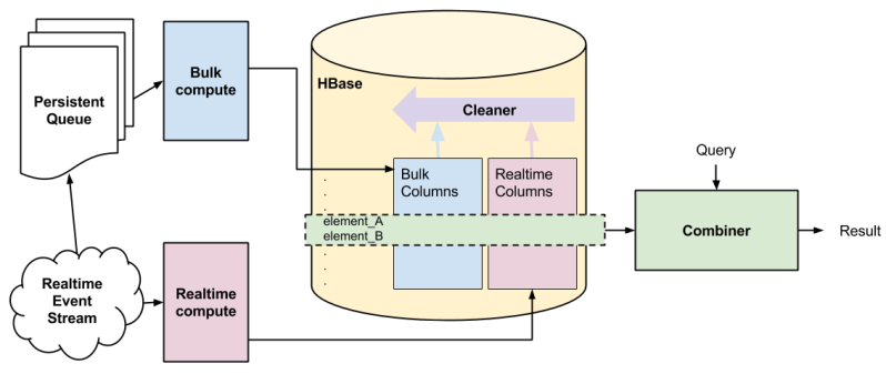
Figure 3. Magic View Architecture

Figure 3 shows an overview of the system and our enhanced Lambda architecture. For the purposes of this discussion, a convenient abstraction is to consider that each row in the HBase table represents the current state of a given photo. The combiner stage is abstracted into a single Java process, which collects data from HBase and runs transformations on the data and sends it to a Redis cache which is used by the serving layer for the site.

Consistency on read in HBase — the combiner

We have two sets of columns to go with each row in HBase: bulk and real time. The combiner determines the final value for each attribute at read. In the case where data exists for real time but not for bulk (or vice versa) then there is only one value to choose. In the case where they both exist we always choose the real time value. This keeps the combiner very simple and fast.

There is a trick though – whenever we do a backfill, we may need to repair the row since the backfill data may be newer than any real time data that is already present. It turns out this slows down the backfill from seven hours to about 14 — still far faster than loading with read-modify-write.

Production throughput

At scale, this architecture has been able to keep up very comfortably with production load. We can simultaneously run backfills to HBase and serve user information at the same time without impacting latency or the user experience.

User experience

An important measure for how the system works is how the viewer perceives it. The slowest part of the system is paging data from HBase into the serving cache; median time for above-the-fold latency – i.e. enough data is available to render the page – is around 10ms.

Future directions

Our experience has been very positive so far with Magic View and we’re looking at how we might enable users to browse their photos in other dimensions (location or color for example). Early tests have shown that building an OLAP or data cube in this architecture is certainly possible but it’s less clear that it will scale well.

Contributors: Peter Welch, Bhautik Joshi, Hugo Haas, Srinivasan Singanallur, Ayan Ray, Pierre Garrigues, Ben Firestone, Sai Madhavan, Tim Miller

Thanks to Nathan Marz for reviewing this post.