Personalized Group Recommendations on Flickr

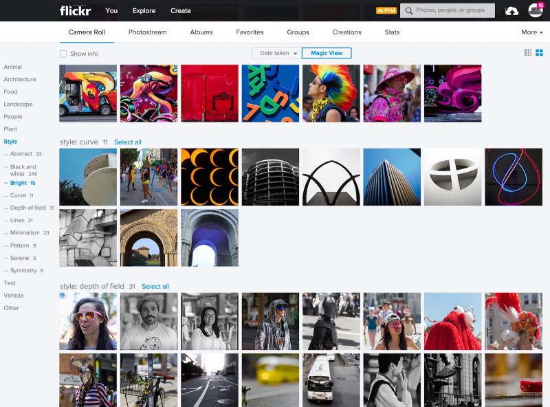
There are two primary paradigms for the discovery of digital content. First is the search paradigm, in which the user is actively looking for specific content using search terms and filters (e.g., Google web search, Flickr image search, Yelp restaurant search, etc.). Second is a passive approach, in which the user browses content presented to them (e.g., NYTimes news, Flickr Explore, and Twitter trending topics). Personalization benefits both approaches by providing relevant content that is tailored to users’ tastes (e.g., Google News, Netflix homepage, LinkedIn job search, etc.). We believe personalization can improve the user experience at Flickr by guiding both new as well as more experienced members as they explore photography. Today, we’re excited to bring you personalized group recommendations.

Flickr Groups are great for bringing people together around a common theme, be it a style of photography, camera, place, event, topic, or just some fun. Community members join for several reasons—to consume photos, to get feedback, to play games, to get more views, or to start a discussion about photos, cameras, life or the universe. We see value in connecting people with appropriate groups based on their interests. Hence, we decided to start the personalization journey by providing contextually relevant and personalized content that is tuned to each person’s unique taste.

Of course, in order to respect users’ privacy, group recommendations only consider public photos and public groups. Additionally, recommendations are private to the user. In other words, nobody else sees what is recommended to an individual.

In this post we describe how we are improving Flickr’s group recommendations. In particular, we describe how we are replacing a curated, non-personalized, static list of groups with a dynamic group recommendation engine that automatically generates new results based on user interactions to provide personalized recommendations unique to each person. The algorithms and backend systems we are building are broad and applicable to other scenarios, such as photo recommendations, contact recommendations, content discovery, etc.

Group_recommendations2.png

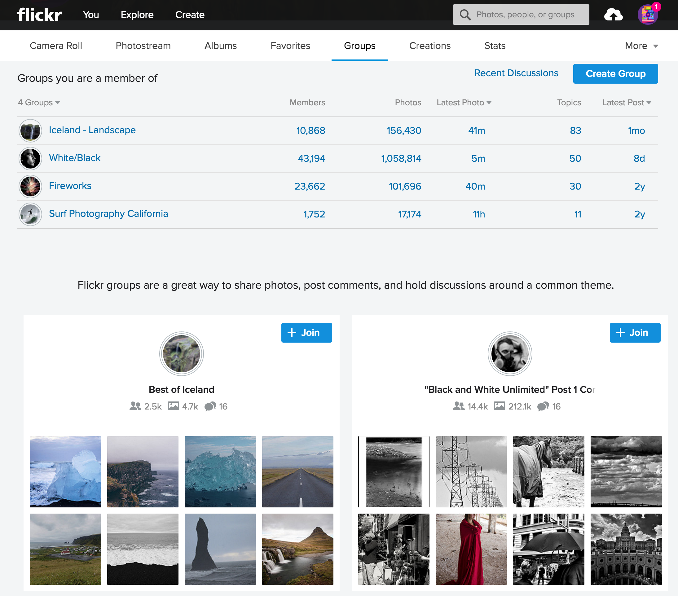
Figure: Personalized group recommendations

Challenges

One challenge of recommendations is determining a user’s interests. These interests could be user-specified, explicit preferences or could be inferred implicitly from their actions, supported by user feedback. For example:

  • Explicit:
    • Ask users what topics interest them
    • Ask users why they joined a particular group
  • Implicit:
    • Infer user tastes from groups they join, photos they like, and users they follow
    • Infer why users joined a particular group based on their activity, interactions, and dwell time
  • Feedback:
    • Get feedback on recommended items when users perform actions such as “Join” or “Follow” or click “Not interested”

Another challenge of recommendations is figuring out group characteristics. I.e.: what type of group is it? What interests does it serve? What brings Flickr members to this group? We can infer this by analyzing group members, photos posted to the group, discussions and amount of activity in the group.

Once we have figured out user preferences and group characteristics, recommendations essentially becomes a matchmaking process. At a high-level, we want to support 3 use cases:

  • Use Case # 1: Given a group, return all groups that are “similar”
  • Use Case # 2: Given a user, return a list of recommended groups
  • Use Case # 3: Given a photo, return a list of groups that the photo could belong to

Collaborative Filtering

One approach to recommender systems is presenting similar content in the current context of actions. For example, Amazon’s “Customers who bought this item also bought” or LinkedIn’s “People also viewed.” Item-based collaborative filtering can be used for computing similar items.

collaborative_filtering

Figure: Collaborative filtering in action

By Moshanin (Own work) [CC BY-SA 3.0] from Wikipedia

Intuitively, two groups are similar if they have the same content or same set of users. We observed that users often post the same photo to multiple groups. So, to begin, we compute group similarity based on a photo’s presence in multiple groups.  

Consider the following sample matrix M(Gi -> Pj) constructed from group photo pools, where 1 means a corresponding group (Gi) contains an image, and empty (0) means a group does not contain the image.

matrix1

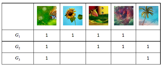
From this, we can compute M.M’ (M’s transpose), which gives us the number of common photos between every pair of groups (Gi, Gj):

matrix2

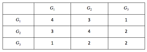
We use modified cosine similarity to compute a similarity score between every pair of groups:

cosinesimilarity

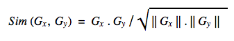
To make this calculation robust, we only consider groups that have a minimum of X photos and keep only strong relationships (i.e., groups that have at least Y common photos). Finally, we use the similarity scores to come up with the top k-nearest neighbors for each group.

We also compute group similarity based on group membership —i.e., by defining group-user relationship (Gi -> Uj) matrix. It is interesting to note that the results obtained from this relationship are very different compared to (Gi, Pj) matrix. The group-photo relationship tends to capture groups that are similar by content (e.g.,“macro photography”). On the other hand, the group-user relationship gives us groups that the same users have joined but are possibly about very different topics, thus providing us with a diversity of results. We can extend this approach by computing group similarity using other features and relationships (e.g., autotags of photos to cluster groups by themes, geotags of photos to cluster groups by place, frequency of discussion to cluster groups by interaction model, etc.).

Using this we can easily come up with a list of similar groups (Use Case # 1). We can either merge the results obtained by different similarity relationships into a single result set, or keep them separate to power features like “Other groups similar to this group” and “People who joined this group also joined.”

We can also use the same data for recommending groups to users (Use Case # 2). We can look at all the groups that the user has already joined and recommend groups similar to those.

To come up with a list of relevant groups for a photo (Use Case # 3), we can compute photo similarity either by using a similar approach as above or by using Flickr computer vision models for finding photos similar to the query photo. A simple approach would then be to recommend groups that these similar photos belong to.

Implementation

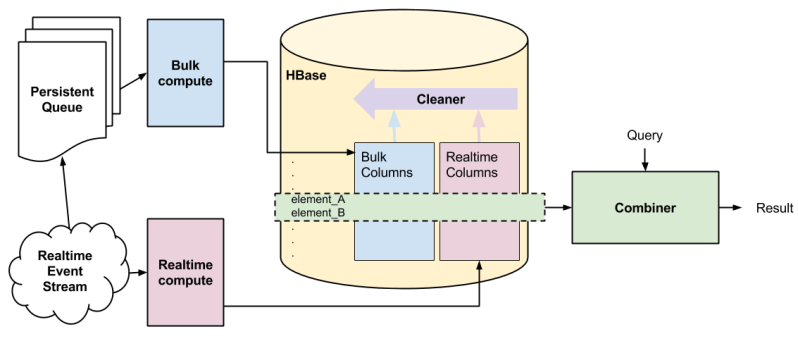
Due to the massive scale (millions of users x 100k groups) of data, we used Yahoo’s Hadoop Stack to implement the collaborative filtering algorithm. We exploited sparsity of entity-item relationship matrices to come up with a more efficient model of computation and used several optimizations for computational efficiency. We only need to compute the similarity model once every 7 days, since signals change slowly.

architecture_diagram

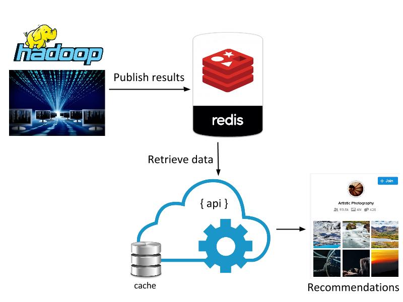
Figure: Computational architecture

(All logos and icons are trademarks of respective entities)


Similarity scores and top k-nearest neighbors for each group are published to Redis for quick lookups needed by the serving layer. Recommendations for each user are computed in real-time when the user visits the groups page. Implementation of the serving layer takes care of a few aspects that are important from usability and performance point-of-view:

  • Freshness of results: Users hate to see the same results being offered even though they might be relevant. We have implemented a randomization scheme that returns fresh results every X hours, while making sure that results stay static over a user’s single session.
  • Diversity of results: Diversity of results in recommendations is very important since a user might not want to join a group that is very similar to a group he’s already involved in. We require a good threshold that balances similarity and diversity. To improve diversity further, we combine recommendations from different algorithms. We also cluster the user’s groups into diverse sets before computing recommendations.
  • Dynamic results: Users expect their interactions to have a quick effect on recommendations. We thus incorporate user interactions while making subsequent recommendations so that the system feels dynamic.
  • Performance: Recommendation results are cached so that API response is quick on subsequent visits.

Cold Start

The drawback to collaborative filtering is that it cannot offer recommendations to new users who do not have any associations. For these users, we plan to recommend groups from an algorithmically computed list of top/trending groups alongside manual curation. As users interact with the system by joining groups, the recommendations become more personalized.

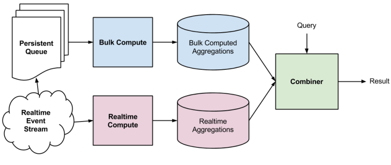
Measuring Effectiveness

We use qualitative feedback from user studies and alpha group testing to understand user expectation and to guide initial feature design. However, for continued algorithmic improvements, we need an objective quantitative metric. Recommendation results by their very nature are subjective, so measuring effectiveness is tricky. The usual approach taken is to roll out to a random population of users and measure the outcome of interest for the test group as compared to the control group (ref: A/B testing).

We plan to employ this technique and measure user interaction and engagement to keep improving the recommendation algorithms. Additionally, we plan to measure explicit signals such as when users click “Not interested.” This feedback will also be used to fine-tune future recommendations for users.

measuringeffectiveness

Figure: Measuring user engagement

Future Directions

While we’re seeing good initial results, we’d like to continue improving the algorithms to provide better results to the Flickr community. Potential future directions can be classified broadly into 3 buckets: algorithmic improvements, new product use cases, and new recommendation applications.

If you’d like to help, we’re hiring. Check out our jobs page and get in touch.

Product Engineering: Mehul Patel, Chenfan (Frank) Sun,  Chinmay Kini

Powering Flickr’s Magic view by fusing bulk and real-time compute

Try it for yourself!

You can try out Flickr’s Magic View on your own photos here, and you can download a working code sample of the simplified lambda architecture here: https://github.com/yahoo/simplified-lambda

Introduction

In this post we’re going to talk about how we came up with a novel revision of the Lambda Architecture for fusing large-scale bulk compute with streaming compute to power Flickr’s Magic View. We were able to create a responsive, real time database operating at a scale of tens of billions of records, with tens to hundreds of millions of records updated per day. We turned to Yahoo’s Hadoop stack to find a way to build this at the massive scale we needed.

Magic View

Figure 1. Magic View in action

Motivation: the Magic View

Flickr’s Magic View takes the hassle out of organizing your photos by applying our computer-vision technology to automatically recognize objects or styles in your photos and present them to you in the Camera Roll’s scrolling view. This all happens in real time as soon as a photo is uploaded, it is categorized and placed into the Magic View.

Aggregating computer vision tags

When a photo is uploaded, it is processed by a computer vision pipeline to generate a set of computer vision tags, which are text labels of the contents of the image. We already had an existing architecture for stream computation of tags on upload, but to implement the Magic View, we needed to maintain per-user reverse indexes and some aggregations of the tags. And we needed to make sure all the data was consistent if a photo was added, removed or updated these indexes and aggregations would have to be updated to reflect this. Finally, we needed to initialize the system with tags for 12 billion photos and videos and run periodic backfills (every time we improved our computer vision algorithms and to cover cases where the stream compute missed images).

The Problem

We initially computed a snapshot of the Magic View indexes and aggregations using map-reduce (via Apache Oozie and Apache Pig), and we were happy with the quick turnaround time (about 7 hours). We considered updating Magic View as a daily batch job, but soon realized this would not give our users the responsive, “live” experience we wanted. So, we built a streaming data layer using Apache Storm and were soon able to update the categories in Magic View in real-time.

The next time we needed to run a backfill, we explored using this streaming layer to load the data. Unfortunately, the overhead of the read-modify-write process was simply too much for a load of this size — after kicking off the process we estimated it would take 28 days this way — much longer than the seven hours we had achieved with a bulk load.

Twenty-eight days was a non-starter – we realized we needed a way to update our bulk aggregations independently of the real-time data streaming in. Solving this problem is how we arrived at our revision to Lambda Architecture. Before digging into the solution, let’s do a quick review of the Lambda Architecture.  If you’re already familiar with it, you can skip this next section.

The Lambda Architecture

We’ll start with Nathan Marz’s book ‘Big Data’, which proposes the database concept of  ‘Lambda Architecture.’ In his analysis, he states that a database query can be represented as a function – Query – which operates on all the data:

result = Query(all data)

In the Lambda architecture, a traditional database is replaced with both a real time and a bulk database. Then query function becomes a “combiner” function of independent queries to each database:

result = Combiner(Query(real time data) + Query(bulk data))

An example of a typical Lambda Architecture is shown in figure 2. It is powered by an append-only queue for its system of record, which is fed by a real time stream of events. Periodically, all the data in the queue is fed into a bulk computation which pre-processes the data to optimize it for queries, and stores these aggregations in a bulk compute database. The real time event stream drives a stream computer, which processes the incoming events into real time aggregations. A query then goes via a query combiner, which queries both the bulk and real time databases, computes the combination, and stores the result.

Typical Lambda Architecture

Figure 2. Typical Lambda Architecture

While relatively new, Lambda Architecture has enjoyed popularity and a number of concrete implementations have been built. Some significant examples are the distributed analytics platform druid, Twitter’s Summingbird, and FiloDB. These implementations conveniently abstract away the databases behind the query combiner.

A significant advantage with this style of architecture is robustness and fault-tolerance via eventual consistency. If a piece of data is skipped in the real time compute there is a guarantee that it will eventually appear in the bulk compute database.

Criticism of the Lambda Architecture has centred around the complicated nature of the combiner. The combiner incurs a developer and systems cost from the need to maintain two different databases. It can be challenging to make sure both systems give the same result. Merging the two queries can become complicated, and finally, more points of failure may be introduced.

The “Ah-ha” Moment

Back to the problem. The data access layer we used for streaming compute uses the atomic read-modify-write pattern to ensure we write consistent data, one record-at-a-time to Apache HBase (a BigTable-style, non-relational database). Again, since this pattern was so much slower in the backfill case we needed to figure out how to get both consistent updates for streaming and  fast loads of the full dataset. Since our bulk data was static, we realized that if we relaxed the consistency constraint we could just run a fast, streaming, write-only load of the bulk data, bringing the load time back down to hours instead of days.

But how could we get around the consistency requirements? We didn’t want a bulk load to clobber data being written from the real time compute process. The insight was that we could just write bulk and streaming data to different column families in the same HBase row. So we added the concept of real time columns and bulk columns in a single row. Basically, bulk loads write to one set of columns and real time writes go to a different set of columns. Since HBase columns are sparse and data is updated relatively slowly we don’t pay much in storage or IO.

We could  now simplify the equation back to:

result = Combiner(Query(data))

The two sets of columns are managed separately by the real time and bulk subsystems. At query time, we perform a single fetch using the HBase API to get both the bulk and real time data. A separate combiner process assembles the final result.

Implementation

 Magic View backend system overview

Figure 3. Magic View Architecture

Figure 3 shows an overview of the system and our enhanced Lambda architecture. For the purposes of this discussion, a convenient abstraction is to consider that each row in the HBase table represents the current state of a given photo. The combiner stage is abstracted into a single Java process, which collects data from HBase and runs transformations on the data and sends it to a Redis cache which is used by the serving layer for the site.

Consistency on read in HBase — the combiner

We have two sets of columns to go with each row in HBase: bulk and real time. The combiner determines the final value for each attribute at read. In the case where data exists for real time but not for bulk (or vice versa) then there is only one value to choose. In the case where they both exist we always choose the real time value. This keeps the combiner very simple and fast.

There is a trick though – whenever we do a backfill, we may need to repair the row since the backfill data may be newer than any real time data that is already present. It turns out this slows down the backfill from seven hours to about 14 — still far faster than loading with read-modify-write.

Production throughput

At scale, this architecture has been able to keep up very comfortably with production load. We can simultaneously run backfills to HBase and serve user information at the same time without impacting latency or the user experience.

User experience

An important measure for how the system works is how the viewer perceives it. The slowest part of the system is paging data from HBase into the serving cache; median time for above-the-fold latency – i.e. enough data is available to render the page – is around 10ms.

Future directions

Our experience has been very positive so far with Magic View and we’re looking at how we might enable users to browse their photos in other dimensions (location or color for example). Early tests have shown that building an OLAP or data cube in this architecture is certainly possible but it’s less clear that it will scale well.

Contributors: Peter Welch, Bhautik Joshi, Hugo Haas, Srinivasan Singanallur, Ayan Ray, Pierre Garrigues, Ben Firestone, Sai Madhavan, Tim Miller

Thanks to Nathan Marz for reviewing this post.

Flickr September 2014

Like this post? Have a love of online photography? Want to work with us? Flickr is hiring mobile, back-end and front-end engineers, in our San Francisco office. Find out more at flickr.com/jobs.

Optimizing Caching: Twemproxy and Memcached at Flickr

Introduction

Flickr places a high priority on our users’ experience, and a critical part of that experience is the speed of the interface.  Regardless of the client you use to access Flickr, caching the proper data and the speed at which our servers can access cached data is critical to delivering on that quality user experience.  The more effective our caching strategy is, the better the Flickr experience will be for our users.  This is true for all the layers of caching we deploy at Flickr from the photo caches to the process data caches buried deep in the system.  In a previous post, we looked at how regional photo caching improved photo serving time in other countries, in this post we’re going to dive down into the innards of Flickr’s software stack and take a look at how we improved Memcached performance for our backend systems.

Back in the olden days (pre-2014), we accessed our Memcached systems through a mix of direct reads from our web servers and writes through a Flickr-developed proxy.  Our proprietary proxy system, Cerberus, handled a whole host of responsibilities. In addition to Memcached set operations, Cerberus managed database updates, the bulk of our Redis accesses, cache consistencyCerberus Based Memcached Architecture 
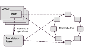
(which is why we directed our writes through Cerberus), and a few other miscellaneous transactions.   As Flickr’s traffic and functionality had grown, Memcached set operation performance wasn’t keeping up, so we needed to consider how to address the gap.

Since the development of Cerberus, the software landscape had drastically changed.  When we developed Cerberus, there was no comparable software available, but now several open source projects exist that provide similar proxy services.  On top of the availability of open source tools, Flickr’s traffic and usage patterns have changed over the course of a decade, changing the requirements we had for a proxy system.  Needless to say we had a lot of questions to ask ourselves before we dived into revising the caching architecture.

After years of operation, we had a good picture into the strengths and weaknesses of our current architecture, so when we started thinking about revising it, a few lessons from the past years really stood out.  One thing that we learned over the years was that Cerberus’ lack of a single purpose made it difficult to troubleshoot operational issues with Memcached.  Due to the lack of isolation, a downstream issue with a user database, could impact Memcached access time.  Whatever came next had to isolate cache requests from other data accesses.

Experience had shown us that Memcached get operation latency was a key performance metric, and we learned through trial and error that placing our current Cerberus proxy between the web servers and the Memcached hosts added more network latency than we were willing to tolerate.  Unfortunately, our options for connection pooling and more efficient use of connections were limited in PHP, so we had little recourse than to suffer with a high connection load and fluctuating connections against our Memcached servers.  The next generation system would have to carefully monitor get operation timings and ensure we didn’t introduce more latency into the process.

So as 2014 rolled around, we started to look into an alternative to Cerberus for accessing the Memcached systems.  Should we build a Cerberus 2.0?  Should we look at an open source alternative?  As we weighed our options, one alternative that stood out because it was quite successful in other parts of Yahoo and throughout the industry was Twitter’s Twemproxy.

Introducing Twemproxy

Twemproxy is a lightweight daemon that proxies requests to a pool of Memcached instances.  It provides the following features that we believed would improve our caching infrastructure:

  • Consistent hashing:  Figuring out what hosts in the ring on which to store and retrieve cache data.  While we had implemented consistent hashing before Twemproxy, it was previously left to the client libraries to sort out.
  • Connection pooling:  Reuse of network connections to the Memcached instances, cutting down significantly on the connection load to the Memcached daemons.
  • Command Pipelining:  Accumulating requests destined for the same host and sending as a combined payload.  This feature further reduces connection load and network overhead to the cache processes.

Resulting Architecture

We implemented a solution where each web server host had two local Twemproxies, forwarding to the Memcached rings.

Twemproxy Based Memcached Architecture

In the resulting architecture, all Memcached operations go through twemproxy.  The change accomplished many goals, including:

  • Providing a dedicated system for Memcached requests that was isolated from other systems
  • Reducing the connection load on our Memcached servers through Twemproxy’s connection pooling.  We experienced a 75% overall reduction of TCP connections to Memcached nodes
  • Improved overall caching latency.  This was a benefit that we didn’t necessarily expect.  With Twemproxy, we found that get operations had a 5% reduction in mean processing time and set operations had a 40% in mean processing time

The Road to Twemproxy

As nice as it would be to say we dropped in Twemproxy, declared victory and went for ice cream, we still had to solve a few interesting challenges along the way: maintaining availability, dealing with disparate consistent hashing schemes, and re-implementing cache coherency.

If One is Good, Two is Even Better

From the start, we recognized that the simple daemon model of Twemproxy would need to be managed carefully.  Each deploy through our continuous deployment system could result in changes to the Memcached hosts configuration.  And unfortunately, configuration changes for Twemproxy require the process to be restarted to take effect.  We measured the time to restart Twemproxy in the 1-2 second range, but even for these necessary restarts, it was too much of an interruption for the clients.

Our solution was to run two instances of the daemon on every host that needed the service and manage a careful synchronization between the restarts.  This restart “dance” was wired into the process that deploys the configuration changes to all the Memcached clients.  A couple of patches have been proposed to allow configuring Twemproxy without restarting it, but none of them have yet made the master branch.

When is Ketama not Ketama?

Ketama is a popular consistent hashing algorithm used by many systems to determine where to place a particular key in a multi-node caching system.  Out of the box, Twemproxy uses an implementation of the Ketama algorithm that is compatible with libketama, the C library which is the most commonly used implementation of the Ketama algorithm.

Our initial implementation of consistent hashing was done using Ketama, but with the Spymemcached Java library.  It turns out that Spymemcached has a slight variation in the implementation that makes it incompatible with Twemproxy.

Our transition from our current system to Twemproxy had to happen live, and a sudden change in the cache algorithm would have a painful (and unacceptable) impact on our database systems.  How could we get across this bridge?  Ultimately, we had to patch Twemproxy’s implementation of Ketama to match Spymemcached to maintain a consistent implementation of the Ketama algorithm.

Redis latency in propagating cache clears

Until we figure out how to change the speed of light, the only way we are going to make Flickr fast across the world, is through multiple data centers conveniently located near our users.  While this is way easier than changing the speed of light, it’s not without its complications.

What do they compute at Night ?

Caches between the data centers have to be kept consistent.  Some caches, like photo caches, deal with immutable data and are easy to keep in synch, others like Memcached systems have read-write data which is harder.  Our approach to handling cache consistency in our Memcached systems was to invalidate stale keys in other colo facilities whenever a process updated a value.  As we mentioned previously, Memcache write operations were directly through our Cerberus proxy specifically so Cerberus could dispatch a cache invalidation event to other colo facilities.  The migration to Twemproxy would not be complete, until we implemented a new solution for cache invalidation.

In our Twemproxy-based architecture, we decided to take the responsibility for cache invalidation our of the hands of the data proxy and push it into the client libraries we used to access Memcached.  Whenever a client updates a Memcache key, it enqueues a corresponding cache invalidation event into a distributed Redis queue.  We then deployed simple, single-purpose Java daemons to process the cache invalidation events from the Redis queue and delete the corresponding keys in their local Memcached systems.  A diagram of the system, appears below: Cache Clear - Blog Post

The wrinkle with this approach was that the enqueuing of clear keys would occasionally take 20 times longer than the normal mean time, pushing cache sets up to 40ms. After much digging, we found that the spikes were happening when the clearing daemons dequeued a batch of keys.  The dequeuing daemons were performing operations across a WAN. Due to the single-threaded nature of Redis, it would periodically block the queue for adding keys for 10s of milliseconds.  Once we figured that out, the fix was a matter of keeping separate in- and out-queues, and moving the keys from in to out with a local daemon, which significantly reduced the blocked time for writing keys.

Conclusion

Caching is crucial to a high-traffic site like Flickr, and we have taken a big stride in making our Memcached utilization more effective.  Using Twemproxy, we were able to clean up an internal system, reduce the connection load on our caching daemons, and even make modest improvements to caching latency for all clients.  Although we faced some technical challenges in implementing twemproxy for Memcached, particularly in propagating cache clear events, it was ultimately well worth the engineering investment.  After several months, our implementation of Twemproxy has proven to make a positive contribution to caching speed and ultimately the experience of a responsive site for our users.

If you dream in low latency and love to rip that extra 10 microseconds of overhead out of an operation, we’d love to have you! Stop by our Jobs page and tell us how awesome you are.